Cache Oblivious Algorithms
Cache-Oblivious Algorithms
Cache-oblivious algorithms seemed incredible to me when I first heard about it in 6.854 (Advanced Algorithms). It’s relatively straightforward to imagine algorithms that utilizes information about page size $B$ and cache size $M$ to create efficient data structures. However, cache-oblivious algorithms are algorithms that achieve similar efficiencies without knowing $B$ or $M$. That means the same cache-oblivious algorithm can be run on computers with different cache or page sizes and still achieve the same asymptotic efficiency as one that is tailored to that specific cache. The key to many of these algorithms is a recursive, fractal-like idea. I’ll describe a cache-oblivious algorithm for searching in a list of integers.
What’s a cache? - The External Memory Model
Here’s the set up. (TLDR at bottom) A program executes on the processor, but the input data resides on the disk. We can think of a disk as a really long linear array of data, but accessing it is really expensive. So, we instead invent this notion of a cache - a layer of memory of $M$ bits that is much smaller, but a lot faster to read/write to. For performance reasons, we will divide the disk and cache into blocks of $B$ bits, called pages, and we will transfer data between cache and disk a page at a time.
This cache sits between the processor and the disk, and the processor will never directly read or write to the disk. When the processor wants to read a piece of data that is not on the cache (this is called a cache miss), it will trigger some mechanism that copies the relevant page from the disk to the cache first, evicting another page if the cache is full, and then read from the cache.
How might this help? Well, trivially, if the entire set of data that the program needs fits in the cache, conceivably the processor could have fetched it all in the cache, paid the one-off cost, and then for the rest of the program the processor will never have to pay the expensive cost of reading from disk. Of course most programs require more data than that, and so we want to design algorithms that minimize cache misses.
Cache management
However, the way computers are set up restricts the tools we have to achieve this. Programs executing on the processor have no explicit control over the cache. Instead, conceptually, programs continue to send read and write requests to the disk as though there is no cache. The processor intercepts these requests, and performs the necessary cache operations to serve the information. In other words, the cache is transparent to programs. Thus, the task of reducing cache misses decomposes into two orthogonal components: writing efficient algorithms by cleverly ordering or specifying memory accesses, and efficient cache management.
For example, an efficient algorithm might try to shuffle memory accesses around so that memory accesses to a particular memory address are clumped together, increasing the likelihood that there will be a cache hit. In fact, because of the paging system, it would doubly help if memory accesses to the same spatial region are clumped together, because there’s a chance they’ll be on the same page.
On the other hand, efficient cache management entails trying to predict which piece of data to evict from the cache when there is a cache miss and we want to load more data into an already full cache. Since we’re focusing on the algorithm this article, we assume that the cache manager has magic oracle powers that lets it discard optimally, so from the algorithm design standpoint, if there exists a sequence of cache loads/writes that achieves our desired performance, we assume that the cache manager will do it. It turns out that this is not unreasonable, because simple techniques such as the Least Recently Used algorithm work really well. (An exposition on this deserves its own article.)
To summarize, the components of the external memory model are:
- Disk, effectively unbounded in size, stores data in pages of size $B$
- Cache, stores $M/B$ pages, each page has size $B$
- Processor executes algorithm, also manages cache.
- Algorithm runs on the processor. When data is needed, the processor transparently loads the required page into the cache if there’s a cache miss, or serve the cached data if there isn’t
There are efficient algorithms that require explicit knowledge of $B$ and $M$, and there cache-oblivous algorithms that are just as efficient, but some how do not. That is to say, the algorithm performs the same actions and requests the same sequence of memory accesses, that works efficiently no matter what size $B$ and $M$ really are. We’ll take a close look at the latter here.
A trivial example: scanning
Let’s say we want to scan through a list of $N$ integers, to do some task, say finding the maximum. If the list occupy a contiguous block of memory on the disk, this can be done efficiently by loading pages one at a time, and scanning through the page before loading the next page. This thus takes $O(N/B)$ disk accesses, and is quite clearly optimal.
Suppose the algorithm does not know $B$. It can achieve the same efficiency by simply reading the elements of the list in order. The CPU will then fetch the first page to the cache, containing elements $0$ to $B-1$ and pass it to the program, and then when the program requires element $B$, it’ll read in the next page, which contains elements $B$ to $2B-1$, possibly overwriting the earlier page. This will just continue until all $N/B$ pages are read. This is cache-oblivious, because the algorithm of sequentially reading the elements is the same regardless of what $B$ is.
Note that in this example, it is essential that the list is stored in a contiguous block of memory. Had the elements been scattered around like in a linked-list, each access could potentially trigger a cache miss, since there’s no guarantee that neighboring elements will be on the same page. This may seem obvious, but this is the main mechanism by which we can write efficient algorithms - coming up with efficient layouts of data.
A puzzle: Searching
Now, let’s consider the problem of searching for an integer in a list. We’ll examine three ways of doing this.
Inefficient cache-oblivious algorithm: Binary search
Let’s assume the data is sorted in a list, and packed contiguously on the disk. A possible algorithm is then to perform binary search, which typically takes $O(\log N)$ reads. The binary search can be viewed a successively narrowing an interval in which the query value may reside in. However, once the interval that the binary search is narrowing is $O(B)$, the entire interval may reside in a page, and no further page accesses are required. Thus, we require only $O(\log N - \log B)$ page accesses. Notice that this is a cache-oblivious algorithm because the algorithm doesn’t know what $B$ is - to the algorithm, it’s just running a standard binary search.
Efficient, but not cache-oblivious: B-trees
Suppose we know $B$ ahead of time. We can achieve $O(\log_B N)$ page accesses. We arrange the list in the format of a B-tree, a generalized BST. Similar to a BST, each subtree of a B-tree corresponds to a contiguous subset of the elements of the list when sorted by value. However, each node $V$ of the tree contains not one, but $B$ elements, which splits the interval corresponding to the subtree rooted at node $V$ into not 2, but $B+1$ intervals. Then, we can traverse down the BST, and each time we go down one level we reduce the interval by a factor of $B$. This thus requires only $O(\log_B N) = O(\log N / \log B)$ page accesses. In reality of course, we have to store pointers and possibly other metadata in each node, so we can’t have exactly $B$ elements in each node, but we can definitely split by $\Theta(B)$ each level.
Efficient cache-oblivious algorithm: van Emde Boas layout
Now we come to the exciting part. We claim that we can achieve $O(\log_B N)$ page accesses, but without having to know $B$ ahead of time. The data structure we’re using is a good old balanced Binary Search Tree. However, the order in which we store the nodes in memory matters. If we pack the the BST in a regular fashion, say in breadth-first order, we could potentially have a situation where almost every vertex in a BST search path, except for the first few, lies in a different page, and thus we’ll have to use $O(\log N - \log B)$ page accesses. The van Embde Boas layout is basically a clever way of ordering the vertices of a binary search tree in a recursive, fractal-like manner such that each page access will fetch the next few vertices that will be queried, so that the next few accesses will be contained within that page.
Concise definition
One application of the recursive van Embde Boas layout
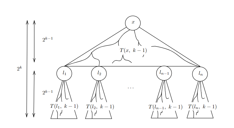
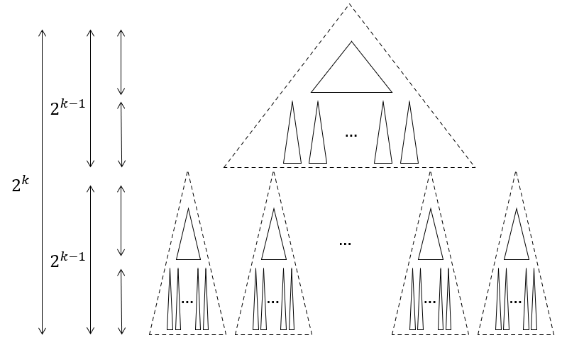
For convenience, suppose the binary tree is complete and has height $H=2^K$. The layout is a permutation of the vertices of the binary tree. Denote $T(x, k)$ as the subtree of height $2^k$, rooted at vertex $x$. If the subtree at $x$ is deeper than $2^k$, then $T(x,k)$ will be the subtree truncated to the required depth. Denote $L(x, k)$ as the layout for that subtree. Then, for some root vertex $x$, of a (sub-)tree with height $h=2^k$, $L(x, k)$ is defined recursively as:
$$L(x, k) = L(x, k-1) \circ L(l_1, k-1) \circ L(l_2, k-1) \circ \dots \circ L(l_{n}, k-1)$$
Where, $l_1, \dots, l_{n}$ are the $n=2^{h/2}$ children of the leaves of $T(x, k-1)$, and $\circ$ is just concatenation. One application of this recursion is shown above.
Visual sketch
If you didn’t catch that, don’t worry about it. Here’s a walkthrough. Suppose we’re given a complete binary tree of height $h=2^k$, rooted at $x$. We want to compute $L(x, k)$, which is a permutation of the vertices in this binary tree. Here’s how it’s done:
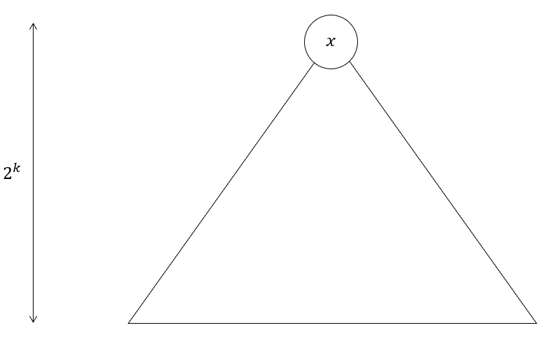
Initial tree
- Cut all the edges between the $2^{k-1}$-th and $2^{k-1}+1$-th layer. This gives us:
- $2^{h/2}$ smaller BSTs with height $2^{k-1}$. These are the children subtrees now disconnected from the main subtree, rooted at vertices $l_1$ to $l_n$, where $n=2^{h/2}$
- One more BST with height $2^{k-1}$, which is the what’s left of the main subtree, now truncated in depth
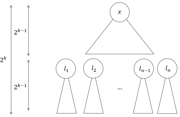
Partition tree
- Apply recursive procedure $L(\cdot, k-1)$ to obtain layouts for each of the $n + 1$ BSTs
- Concatenate the layouts and return (the order doesn’t actually matter)
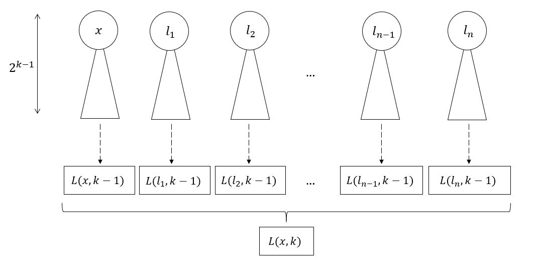
Concatenate sub-layouts
Sierpinski triangles, atoms and time
Now this tells us how to construct the layout, but it’ll be more helpful to develop some intuition about what this layout looks like.
An intuitive way to look at this is to draw analogy to the Sierpinski triangle, which can be constructed by repeatedly applying the same partitioning procedure to a full triangle. We can view successive partitioning as an evolution in time. Similar to the Sierpinski triangle, the layout partitions the subtree into smaller subtrees, and then recursively applies the same procedure to each smaller subtree.

Evolution of Sierpinski Triangle (Wikimedia Commons)
This analogy gives us some insights. Recursion is typically viewed as a depth-first process, as most programming languages implement it that way. This leads us to instinctively follow a recursion branch deeper and deeper, but this doesn’t really give us the intuition we need to understand this. Instead, we can adopt the perspective that the Sierpinsiki triangle gives, and we instead limit the recursion depth. This is akin to expanding the recursion in a breadth-first rather than a depth-first manner.
To put things concretely, let $t$ be the recursion depth limit. We introduce a term ‘atom’ for the subtree unit that the recursion partitions into at depth $t$. For $t=0$, the recursion is completely unexpanded, and the atom is the whole tree. Quite trivially, all vertices in this atom are placed in a contiguous range in the final layout.
Recursion depth is 0. The atom is the whole tree
Next, to step into $t=1$, we evaluate one layer of the recursion. The atoms are now subtrees of height $2^{k-1}$. The concatenation process joins the layouts of the individual atoms, so we can safely say that in the final layout, all vertices in the same atom are in a contiguous segment. Notice that for this property to hold, it doesn’t matter which order we joined the layouts of the atoms in as long as we don’t break an atom up.
Recursion depth is 1. The atoms are subtrees of height $2^{k-1}$
Now, we evaluate one more layer of the recursion for $t=2$. The atoms are now subtrees of height $2^{k-2}$. For the same reasoning as before, in the final layout, all vertices in the same atom are in a contiguous segment.
Recursion depth is 2. The atoms are subtrees of height $2^{k-2}$
And this process continues until the atoms are individual vertices. Thus, if we limit the recursion depth, we can view the recursive calls to the layout as successively partioning the tree into finer and finer atoms. More precisely, in the evolution for the van Embde Boas layout, after applying $t$ levels of recursive calls, all vertices are partitioned into subtrees of height $2^{K-t}$. This perspective lets us say something powerful about the atoms:
In the final layout, we can choose any resolution to look at the layout. All vertices in any atom at this resolution will be in a contiguous segment.
Algorithm
At this point, you might already have a pretty good idea of what the algorithm is. Given this layout, the cache-oblivious algorithm is the straightforward algorithm that traverses down this BST. Now, let’s analyze more formally why this is efficient.
Suppose the page size is $B$. Every time step, the height of atoms halves. We’re interested in the height of the atoms at the first time step where an entire atom can fit in a page. Since the number of vertices in a complete binary tree grows exponentially with height, that happens when atoms have height $\Theta(\log B)$. Then, analysing the layout at this resolution, we can fit any atom (which all have the same height of $\Theta(\log B)$) into the cache with 1 page load*.
Then, now consider what happens in a search. A search basically consists of a path from the root of the BST to some leaf*. This path will spend some time in the first atom, until it reaches the leaf of the atom and goes into the next atom, and so forth. Since the path always start at the root vertex of an atom and ends on a leaf, it will spend $\Theta(\log B)$ steps in that atom. Since the overall search path is $\log N$ steps long, we’ll need $O(\frac{\log N}{\log B}) = O(\log_B N)$ atoms, and that’s the number of page accesses we need.
Remarks
The heart of the algorithm is the fractal nature of the van Embde Boas layout, which gives some kind of scale invariance. This idea of geometric scaling is actually a pretty common argument in algorithm analysis, but I find this particular instance incredibly visual and vivid. I was guilty of cutting a few corners here, and I’ve marked some of the more egregious parts with an asterix. Nonetheless, I hope I was able to convey the main intuition in this article and if you’re interested in the details I glossed over or reading more about cache-oblivious algorithms, I’d recommend Erik Demaine’s awesome and accessible review paper.
Edit: hacker news discussion